 Github Repository
Durchhang eines flexiblen Kabels
Contents
Voraussetzungen
mathematische Grundlagen von Randwertproblemen
Reduktion von ODEs höherer Ordnung
Bisektionsverfahren
Lerninhalte
Implementierung einer Routine zum Lösen von Randwertproblemen mittels Schießverfahren
Durchhang eines flexiblen Kabels
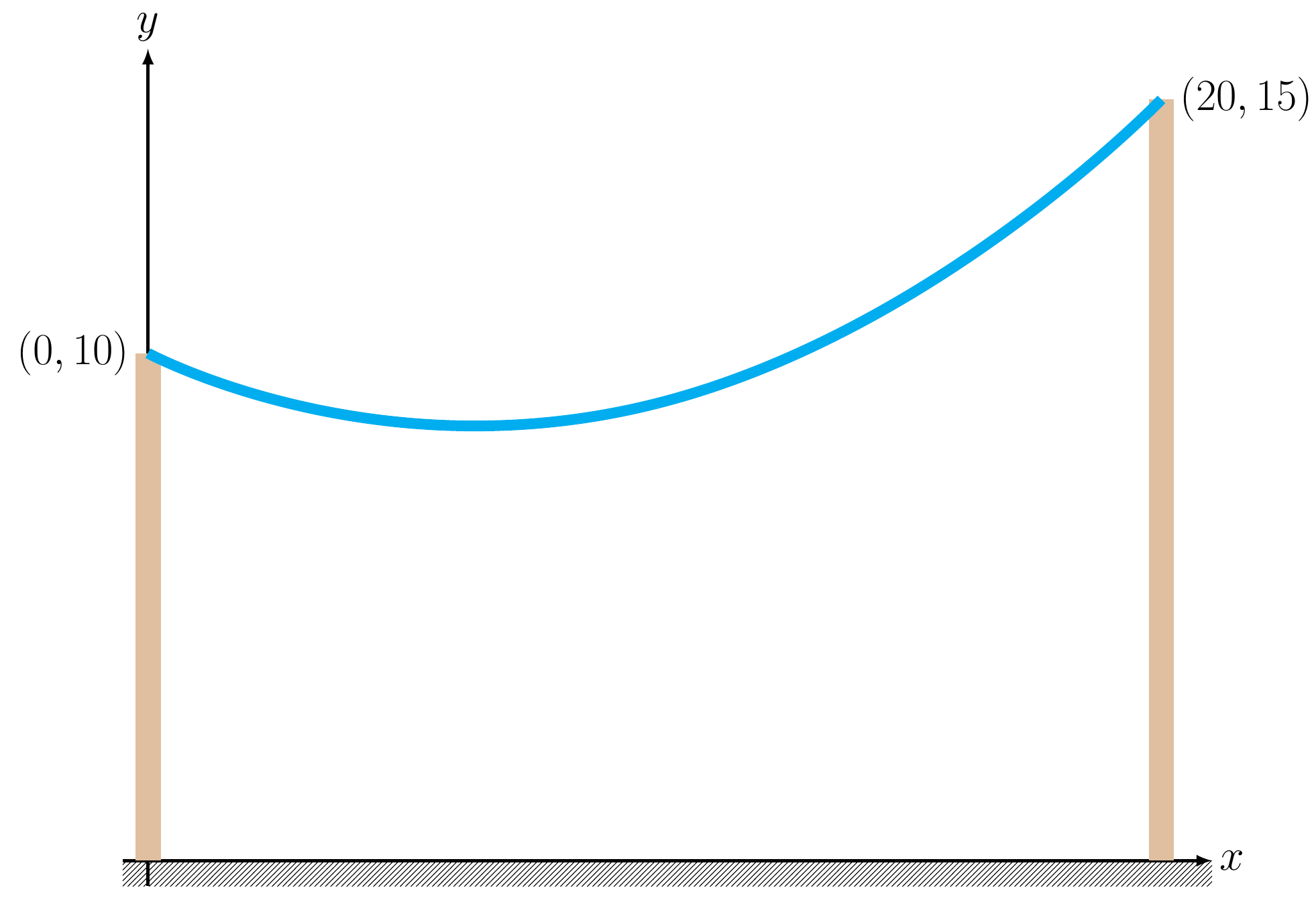
Ein flexibles Kabel einheitlicher Dichte ist an zwei Punkten \(y(0) = 10\;\mathrm{m}\) und \(y(20) = 15\;\mathrm{m}\) aufgehängt. Die Form des Kabels folgt der Differentialgleichung
wobei \(C=0.041\;\mathrm{m}^{-1}\) eine Konstante ist, die das Kabelgewicht pro Einheitslänge sowie den horizontalen Spannungsanteil im tiefsten Punkt des Kabels enthält.
Aufgabe 1
Verwenden Sie die Matlab-Routine bvp4c um den Verlauf des Kabels zwischen \(x = 0\;\mathrm{m}\) und \(\mathrm{x} = 20 \;\mathrm{m}\) zu bestimmen.
Aufgabe 2
Lösen Sie das Randwertproblem nun mit dem so genannten Schießverfahren. Wählen Sie hierzu zwei Schätzungen für die unbekannten Ableitungen \(\frac{\mathrm{d}y}{\mathrm{d}x}\) bei \(x=0\). Schießen Sie auf \(x=20\), indem Sie die Differentialgleichung als Anfangswertproblem mit ode45 für beide Schätzwerte \(\frac{\mathrm{d}y}{\mathrm{d}x}\) lösen. Vergleichen Sie die getroffenen \(y(x=20)\)-Werte mit dem Zielwert \(y(x=20)=15\). Wenn eine Ihrer Schätzungen den Zielwert unterschätzt, und die andere den Zielwert überschätzt, können Sie sich mittels Bisektionsverfahren dem tatsächlichen Wert für \(\frac{\mathrm{d}y}{\mathrm{d}x}(x=0)\) nähern. Führen Sie eine Bisektion durch, um sich dem Zielwert bis auf tol \(= 0.01\;\textrm{m}\) zu nähern.
%%file bvpsm.m
function sol = bvpsm(odefun, x, ybc, yp_lower, yp_upper, tol, max_iter)
% this functions solves a boundary value problem with dirichlet boundary conditions using
% the shooting method.
%
% Internally, the bisection method is used to dermine the slope af the left boundary.
%
% INPUTS:
%    - odefun is a function handle  for the right-hand side of the scalar ode
%      of second order y'' = f(t,y,y').
%    - x=[xa, xb] is a 1x2 vector containing the start and end value for the interval, on
%      on which the BVP is to be solved
%    - ybc=[ya, yb] is the a 1x2 vector containing the Dirichlet boundary conditions of the BVP.
%    - yp_lower is a lower estimate of the slope of y and yp_upper is an upper estimate of the
%      slope of y at xa. These values are needed by the shooting method.
%    - tol is a tolerance for the right boundary condition. The problem is considered as solved,
%      if abs(y(xb)-yb) < tol
%    - max_iter are the maximum number of iterations for determining the slope at xa
%
% OUTPUTS:
%    - sol is the solution structure, as it is returned by the initial value problem solvers
%      such as ode45

% PUT YOUR IMPLEMENTATION HERE
Hinweis
In dem Kapitel Skripte und Funktionen wurde eine Funktion für das Bisektionsverfahren entwickelt. Verwenden Sie diese Funktion in Ihrer Implementierung, um das Rad nicht neu erfinden zu müssen.
% SPACE FOR SOLUTION: Apply the function bvpsm to solve the BVP of the flexible cable.