 Github Repository
Newton-Verfahren
Contents
Voraussetzungen
mathematische Grundlagen von
Newton-Verfahren
Jacobi-Matrix
finite Differenzen
Lerninhalte
Implementierung und Anwendung des mehrdimensionalen Newton-Verfahrens als selbst erstellte Routine
Newton-Verfahren
Aufgabe 1

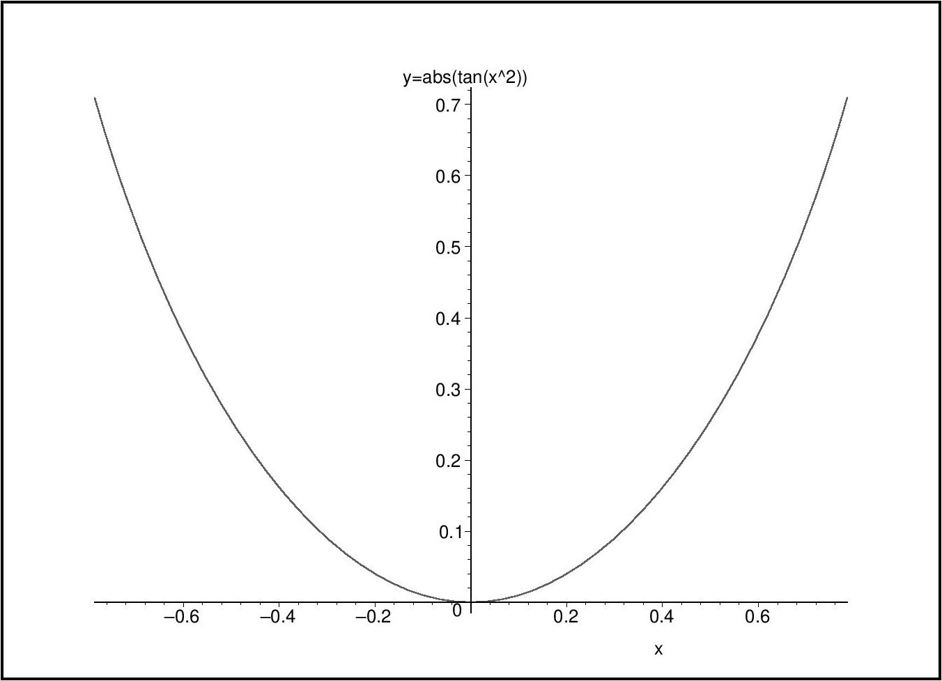
Gegeben sei ein Weinglas mit dem Querschnitt \(y= tan(x^2)\). An welcher Stelle auf der y-Achse muss der Eichstrich für einen Inhalt von \(V=0.5\) gezogen werden?
Hinweis
Um das Volumen auszurechnen, können Sie das Glas auch als Rotationskörper um die x-Achse ansehen.
\[V=\pi \cdot \int _{a}^{b}(f(x))^{2}\mathrm {d} x\]Die Stammfunktion von \(\arctan(x)\) ist:
\[x\arctan \left( x \right) -1/2\,\ln \left( 1+{x}^{2} \right)\]
Verwenden Sie zur Lösung die Matlab-Funktion fzero.
Aus der Hilfe zu fzero:
FZERO  Scalar nonlinear zero finding.
X = FZERO(FUN,X0) tries to find a zero of the function FUN near X0,
if X0 is a scalar.
Examples
   FUN can be specified using @:
   X = fzero(@sin,3)
   returns pi.
% SPACE FOR SOLUTION
Aufgabe 2
Zum Finden einer Nullstelle implementieren Sie nun das Newton-Verfahren. Angefangen mit einem Startwert \(\mathbf{x}_{0}\) muss in jeder Iteration folgende Verfahrensvorschrift erfüllt werden:
a) Programmieren Sie das Newton-Verfahren, so dass es wie fzero angewendet werden kann. Da die Ableitung der Funktion noch sehr einfach von Hand zu berechnen ist, kann sie dem Programm übergeben werden.
Hinweis
Machen Sie sich mit Function Handles und Anonymous Functions in Matlab vertraut.
%%file simple_newton.m
function x = simple_newton(func,deriv,x0,tol,maxit)
% z = simple_newton(f,df,x0,tol,maxit) solves the nonlinear system 0=func(x)
%
% inputs:
%   func    a handle to the nonlinear function
%   deriv   a handle to the derivative of the nonlinear function
%   x0      initial guess for the Newton method
%   atol    absolute tolerance
%   maxit   maximum number of Newton iterations

% YOUR CODE HERE
Das erstellte Programm lässt sich folgendermaßen testen:
moxunit_runtests test_simple_newton.m
b) Lösen Sie Aufgabe 1 noch einmal mit Hilfe Ihres soeben programmierten Newton-Verfahrens und schauen Sie, ob die Ergebnisse übereinstimmen.
% SPACE FOR SOLUTION
Aufgabe 3
Gegeben sei das nichtlineare System
und eine Lösung für \(x\) liegt in der Nähe von
a) Bestimmen Sie die Jacobimatrix des Systems.
Um dem Newton-Verfahren nicht jedes mal eine Jacobi-Matrix übergeben zu müssen, kann diese auch mittels finiter Differenzen approximiert werden. Das hat den Vorteil, dass so auch komplexe Systeme einfach gelöst werden können. Aufgrund der Approximierung verlieren wir aber an Genauigkeit.
b) Schreiben Sie eine Matlab-Funktion, die die Jacobimatrix \(J_F(\mathbf{x})\) für eine beliebige Funktion \(F:\mathbb{R}^n \to \mathbb{R}^m\) mit Differenzenquotienten (“finiten Differenzen”) approximiert. Dabei soll die Eingabe F ein Function Handle einer beliebigen Funktion sein, beispielsweise @sin oder in diesem Fall @(x) [5*x(1)^2-x(2)^2; x(1)*x(2)-1/4*(sin(x(1))+cos(x(2)))+1/4]. x ist hierbei der Vektor, an dem die Matrix ausgewertet werden soll und wird als [1/8; 1/4] übergeben.
Hinweis
Sie können Ihr Programm in der Aufgabe Aufgabe 2: Das Newton-Verfahren wiederverwenden. Speichern Sie Ihre Lösung also bestenfalls nach der Fertigstellung ab.
Implementieren Sie eine Schleife über die Spalten der Jacobi-Matrix, pro Spalte müssen Sie einen Differenzenquotienten bilden.
Ihr Programm sollte mit \(n+1\) Funktionsaufrufen von
Fauskommen.Achten Sie darauf, dass alle Funktionen \(F:\mathbb{R}^n \to \mathbb{R}^m\) auf die Sie die
jacobianFunktion anwenden Spaltenvektoren auf Spaltenvektoren abbilden.
%%file jacobian.m
function J = jacobian(F,x)
% J = jacobian(F,x) returns the (m x n) Jacobian matrix of F evaluated at x
%
%   |  dF1/dx1 ... dF1/dxn |
%   |     .           .    |
%   |  dFm/dx1 ... dFm/dxn |
%
% It uses finite difference approximations. x must be a (n,1)-column vector and F must be a function
% taking an (n,1)-vector as an input. m is deduced from F.

% YOUR CODE HERE
Prüfen Sie nun mit Hilfe Ihrer in a) errechneten Jacobimatrix die Ergebnisse für verschiedene x. Sie können Ihr Programm des Weiteren auch mittels eines Unit Tests überprüfen:
moxunit_runtests test_jacobian.m
b) Erweitern Sie mit Hilfe des zuvor erstellten Programms zur Auswertung der Jacobimatrix Ihr Programm für das Newton-Verfahren, sodass es nun das oben genannte Gleichungssystem lösen kann.
Hinweis
Sie können Ihr Programm in der Aufgabe Aufgabe 2: Das Newton-Verfahren wiederverwenden. Speichern Sie Ihre Lösung also bestenfalls nach der Fertigstellung ab.
%%file newton.m
function z = newton(func,z0,tol,maxit)
% z = newton(F,z0,tol,maxit) solves the nonlinear system 0=func(z)
%
% inputs:
%   func    a handle to the nonlinear function
%   z0      initial guess for the Newton method
%   atol    absolute tolerance
%   maxit   maximum number of Newton iterations

% YOUR CODE HERE
Auch dieses Programm lässt sich mittels eines Unit Tests überprüfen:
moxunit_runtests test_newton.m
Ermitteln Sie nun die Lösung des oben genannten Gleichungssystems:
% solve nonlinear function for x
x = newton(@(x) [5*x(1)^2-x(2)^2; x(1)*x(2)-1/4*(sin(x(1))+cos(x(2)))+1/4],[1/8; 1/4],eps,100)
Zur Kontrolle berechnen wir das Gleichungssystem nochmal rückwärts.
Erinnerung:
% check if solution solves the nonlinear system
y = [5*x(1)^2-x(2)^2; x(1)*x(2)-1/4*(sin(x(1))+cos(x(2)))]
if max(abs(y-[0;-1/4])) > eps
    disp(['Incorrect solution with a tolerance of |', num2str(max(abs(y-[0;-1/4]))), '| > eps'])
else
    disp(['Correct solution with a tolerance of |', num2str(max(abs(y-[0;-1/4]))), '| <= eps'])
end